
A Rationale
Perhaps you are a college faculty member and want to know if something you are doing in the classroom is improving student outcomes in your class. Perhaps you are a member of leadership and want some analysis of departmental or college-wide initiatives to evaluate their impact on student learning. Perhaps you have a systems background and are just interested. There are a variety of use cases for building databases and using statistical packages to analyze them.
This paper is intended to provide some ideas and examples of how to accomplish your analytical goals. The specific tools you may ultimately select may be different, but at the least, this paper can help set a framework for how to approach the problem of collecting and analyzing data.
How To Get Started
The first item on your to do list should be a project plan that identifies the goal of your project. For example: “I want to use a linear regression to evaluate the impact of a teaching technique on student learning” or “I want to build a preference score match statistical model to analyze the impact of a change in textbooks on student learning.”
Next, take some time to consider where you might collect data for your analysis. Does your institution provide access to data via a comma separated file (csv)? Can your colleagues contribute data via Excel? Do you have access to a data warehouse on a SQL Server or Oracle database system? Will you need to gather some data manually?
Next, consider what data you need to develop your analysis. For educational research, you may need access to a variety of categorical data to be able to control for natural variation in student outcomes based on student-specific or instructor-specific variations. Alyahyan and Dustegor (2020) identified numerous factors that may correlate with student success, including (a) past student performance such as high school grade point average and/or student grade point average in prior college courses; (b) student demographics such as gender, race, and socioeconomic status; (c) the type of class, semester duration, and program of study; (d) psychological factors of the student such as student interest, stress, anxiety, and motivation; and (e) e-learning data points such as student logins to the LMS and other student LMS activity. You also should give due regard to the sample size you may need to be able to generalize your analysis.
Next, consider what tools you may need for data collection and analysis. This paper discusses several tools that you may wish to use, such as the statistical package, R, a database application, MySQL, and a scripting language that would permit the import and pre-processing of raw data into your research database, Python. You may also need a way to manually collect data, perhaps by implementing a website that connects to your database through a server-side scripting language like php, or by designing a basic data collection instrument in Excel. Other tools for collecting surveys, such as SurveyMonkey or Microsoft Forms, may also be helpful. Many of the above tools are open source and freely available by researchers, but some may not fit your particular computing environment, or they may not work in exactly the same way as discussed in this paper.
Finally, the reader should also take into account whether your planned research may require Institutional Review Board (IRB) approval. More information is available in 34 CFR § 97; some forms of educational research are exempt (such as the research on the “effectiveness of or the comparison among instructional techniques” at 104(d)(1)) from IRB review, where others (such as surveys of students under (d)(2)) may require some consideration for anonymity or limited IRB review.
The Prerequisites
You may or may not have all of the tools described in this paper already available to you. If not, one method to get them is to use Homebrew, a package manager for MacOS and Linux, available here: https://brew.sh/.
Once Homebrew is installed, you can use this tool at the MacOS Terminal shell prompt to install other packages through a simple command line script:
$ brew install python
$ brew install mysql
$ brew install r
Homebrew will then download and install your tools to a specific directory (older Macs install to /usr/local/opt; Silicon-based Macs use /opt/homebrew). Homebrew will then add these functions to the Terminal path so that you can execute commands by just entering:
$ r
$ python [/path/to/your/python/script/goes/here]
Alternately, you can usually download and use a package installer script that will install tools visually and configure certain default options for you. For example, MySQL has a DMG file you can use to install MySQL: https://dev.mysql.com/doc/refman/8.0/en/macos-installation.html. A bit of searching with your favorite web search tool will help you from here.
You also may or may not be comfortable using the Terminal to interact with your operating system, unless you are a fossil like me and worked with MS DOS 3.1 back when personal computing was still a new idea. If you prefer a graphical user interface, you may need some additional tools that will help you to access and/or analyze your data. For example, HeidiSQL gives you a graphical view of your MySQL databases. R can be installed with a partly graphical user interface (though you will still need to create code for the actual data analysis).
In addition, R and Python may both need you to do some further installation of modules each uses for various tasks discussed in this paper. Python modules can be installed using pip:
$ pip install pandas
$ pip install urllib
$ pip install pymysql
$ pip install datetime
Similarly, R has a command line option to install new packages that you may need within R:
install.packages(“ggplot2”)
install.packages(“RMySQL”)
install.packages(“lmer”)
install.packages(“parallel”)
install.packages(“marginaleffects”)
install.packages(“tidyr”)
Onwards to data analysis!
The Big Picture
Before we dive into specifics, let’s talk about the basic process here for using these tools for your research goals.
Once you have defined the data that you need, you will need to gather that data into one place to conduct your analysis. You have some options for getting your data from institutional sources, export from a learning management system, or manually collecting the data into a simple collection tool in Excel. This paper discusses importing from comma separated values files, but there may be other file formats you may encounter. MySQL itself has a way to import .csv and .xml files natively, though that tool may not be sufficiently flexible for processing your raw data. Python is a more flexible alternative for cleaning up and importing data into a database file, though a bit more patience may be needed to develop and test your code.
Once you have your data, you may be able to begin your statistical analysis in R. In some cases, you may need to define views that include formulas or conditional fields before you can move on to R. This will depend on your specific research questions and the condition of the raw data you processed, and how creative you are with your import process.
From within R, you can conduct a variety of statistical and graphical analyses of your data, using a variety of modules available to R users, such as lm, lmer, matchit, and ggplot.
Data Collection
Perhaps the data is collected for you and made available at your institution in a data warehouse, and by design the data set has the variables you need for your research. If that is your situation – congratulations – you can skip over this section (to the envy of the other readers of this article).
However, you may find that either: (a) you have myriad data sources in various file formats that are not available in one system, (b) the data you do have access to may not be complete or you may need to define specific variables and aren’t able to do that with your remote data source, or (c) you wish to have a copy of this data over which you can exercise control. If any of these fit your situation, or you need to gather data by hand, read on, gentle reader!
One approach is to collect your data in .csv files and import these into a MySQL database table using a MySQL’s load data command or a Python script. For example, if you want to research how things went in courses you taught this semester, you might be able to export your grade books from your courses out of your learning management system and into a .csv file. D2L’s Brightspace and Blackboard both provide an option to do this. Some may instead support export to an Excel spreadsheet, which can then be exported into .csv file format from within Excel’s “Save As” function.
In other cases, your starting point may instead be a .pdf file of your data. Python also has other tools that can be used to import data from .pdf files.
Or, you may have to create a data collection instrument yourself. You can use Excel for basic data collection by defining specific columns of information you plan to manually collect for your research project. For example:

In creating your data collection instrument, you can help yourself by having column names in the first row, though Python can manage if you don’t do this, as long as you remember what data you put where!
Data Import
Once you have your raw data, you again have some options for what to do next. My recommendation is that you import all of your data into a MySQL database, but know that you are free to use a different database solution. If you do, be sure to check that it supports Open Database Connectivity (“ODBC”) and that both Python and R have a way to reach this database to insert and manipulate your raw data, and to query the processed data for analysis later.
For this step to work, two things have to be true. One, you need a place to put the data, and two, you need a way to import your raw data to that place. To accomplish the former, you can create a MySQL database, add user permissions, and create a table that will store your data using Structured Query Language (“SQL”). Assuming that your data is organized as above in the prior example, you could connect to your MySQL server, create a new database and a new table to store your data as follows:
mysql -u root -p (after pressing Enter, the terminal will ask for the password to access your database server locally)
create database mydata; (to make your database)
use mydata; (to switch into this database)
CREATE USER ‘your_user_name’@’localhost’ IDENTIFIED BY ‘password (be creative)’; (I know it feels like I am shouting at MySQL, but I learned that from the internet when creating new user accounts)
GRANT ALL PRIVILEGES ON *.* TO ‘your_user_name’@’localhost’; (give your new user account full permissions on your data table; for database administrators cringing in their chairs, you could also be more specific and just grant SELECT permissions if you are really going to be like that with a GRANT SELECT on mydata.* TO ‘your_user_name’@’localhost’;)
create table tbMyData (dataID NOT NULL AUTO_INCREMENT, StudentID int, FinalGrade char(1), Intervention int, GPA decimal(6,2), Race char(1), Gender char(1), Age int, PRIMARY KEY (dataID) );
Now, that wasn’t so bad, right? Also, all those semicolons are not just me trying to fix a bunch of run-on sentences. MySQL uses the semicolon in its syntax to know when you are at the end of your SQL statement and that it should now execute whatever you have entered.
Before you go any further, be sure to put the password you created above somewhere safe. You will need that later so that R can reach your database.
The next step in your process is to import your data into your freshly created database file. You have some choices here. One possibility is to use the MySQL native load data command. This can work if the table you have created above is organized in the same order as the data in your .csv file that you have diligently created earlier from your institutional data sources or you have collected by hand. In order to load data into MySQL, a few things are needed. First, you need to log in to MySQL using the local-infile=1 switch, as:
mysql –local-infile=1 -u root -p
Next, you need to tell use your database where you wish to import your data, and then tell MySQL you want to load local data into the database with this command:
set GLOBAL local_infile = ‘ON’;
These safety precautions are meant to keep you from harming your innocent data with careless data import processes; for the more data cavalier, these are unjust restrictions on your data import liberties. Either way, you have to tell MySQL you are going to load some data or nothing will happen with the next command in MySQL:
load data LOCAL infile ‘/path/to/your/data/Import.csv’ into table tbMyData FIELDS TERMINATED BY ‘,’ LINES TERMINATED BY ‘\n’ IGNORE 1 ROWS;
The load data command has a variety of options but the obvious here is to take a file you have provided the path to and import it into a table called tbMyData. The remainder of the syntax here is to tell load data the field delimiter (in my case that is a comma, but you could use a pipe or semicolon or anything else you want if you control the file export process; “comma separated values” files assume a comma is the field delimiter), the row delimiter (the “\n” here means a carriage return), and IGNORE 1 ROWS tells load data that your first row has row headers and is not the data itself. You won’t need the latter if you didn’t define any row headers because you are living on the data-edge and prefer to rely on your memory that column 39 contained the student’s Age, while column 14 was the final grade in the course.
Load data won’t work in all situations. In fact, I have created just such a situation in this paper because I created a primary key field as the first field in my table above, but the sample .csv file I created starts instead with the StudentID.
Even if I didn’t manufacture a reason to turn to Python, my experience is that when you are getting data from other sources, these files will contain data that you don’t need to import, or data that needs to be manipulated before you can insert it into your database. Python scripting is a flexible way to address some of these kinds of problems. Before we go on, you might want to grab a cup of coffee or walk the dog, especially for those with command line anxiety syndrome!
Import with Python to MySQL
Python is a flexible scripting language that can reliably import data for your project into your MySQL database. There are some basic parts to the script below that I have broken into sections to help make the script easier to follow. When working in this language, be mindful of your indenting as this tells Python whether a particular block of code belongs with a particular condition, function, loop, or other control structure in your code. Also, comments start with the hash tag, #.
Here are the basic building blocks of code for this project:
- Modules Imported into your Python Script
- Defined functions that begin with “def”
- Database connection variables to reach your MySQL database
- Identify the .csv file you wish to process
- Loop through each row of the .csv file and process each column of data, then
- Insert a record using SQL into your database and commit the record
Ready? Here WE GO!
The Modules you need:

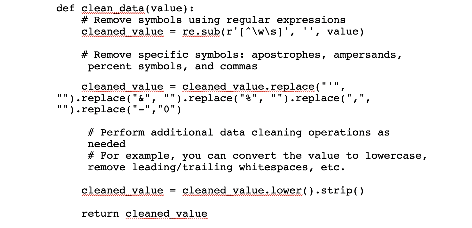
MySQL is weird about the format of dates for insert statements:

I know this is a shock, but sometimes your raw data has weird characters that will cause problems for your code. This function will try to strip out weird stuff so your database doesn’t choke on malformed insert statements further on.
The next portion of the code will define your connection with pandas to your MySQL database:

The remainder of the code will then open a connection to the database, connect through pandas to the .csv file you are importing, fill in default values in fields where data may be missing, and then loop through each row of your file and insert the values into the MySQL database using a constructed SQL statement and executing it with the open MySQL cursor object.
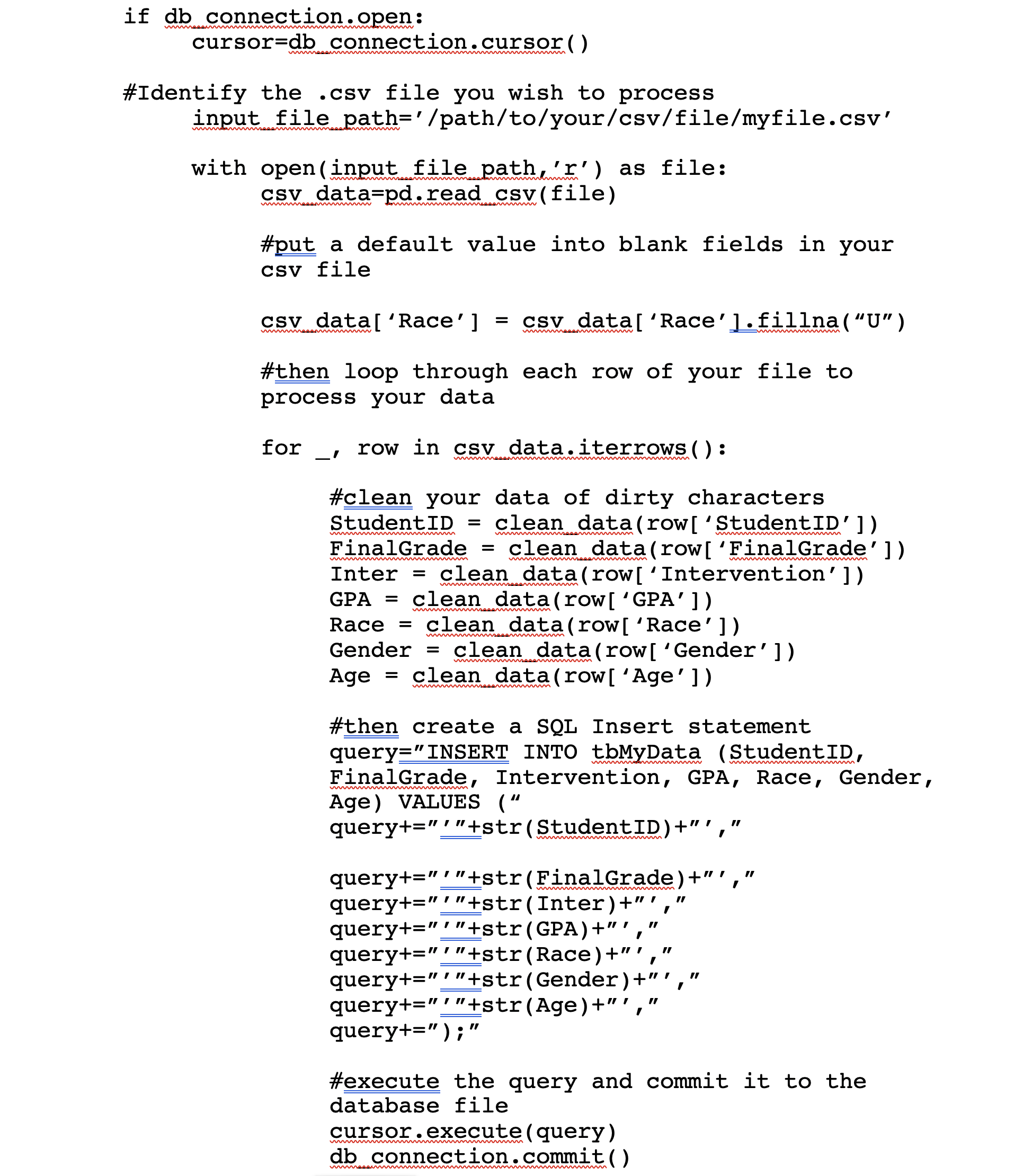
For data junkies that are opposed to header rows on principle, you can also refer to a particular column by its number, starting with the number 0 to mean the first column (obviously – who would start at 1 for the first column?): row[‘0’]
Once you have created your script, save it with a name you can remember, and the extension .py so that everyone will know that this is a python script. Then you can execute it by using a command at the terminal like so:
python /path/to/your/script/script_name.py
And, if we are all living right, python will find your .csv file, roll through each and every row in the file, and insert each one into your database file.
For the rest of us that are living in the sin that is our reality, there may be a problem and python will tell you what row offends its sense of natural order for further troubleshooting. Python tends to get mad at you for having too many or too few indents for blocks of code, and for syntax errors (the period (.) concatenates strings in some languages, whereas plus (+) concatenates in Python). Stay calm and troubleshoot with a cup of coffee and a dose of patience. If you have a particular step with an error, using the print() command to print out information at the command line while the script runs is a method to help troubleshoot errors (such as SQL syntax errors, print(query)).
Now, the above script has to be modified for each file you want to import, which can be a pain if you have many files to process. You can probably find a way to loop through all of the .csv files you want to process in a particular directory with Python and the os module. Extra credit if you can find a method to move processed files out of your import directory using shutil.
So, did your data import? You can check by going over to your MySQL database and executing a query like:
select * from tbMyData;
If things are not as you had hoped, never fear! You can always truncate table tbMydata; and re-run your python script after making adjustments to get things as you need them to be.
Using R for Data Analysis
Well, you have made it this far, kind reader, and I trust that the data journey has treated you well. Your final destination is within your grasp and your dreams of data analysis are on the cusp of being realized! Let’s get started with R!
At the terminal, anti-climatically type the letter R and press enter, and behold!
$ r
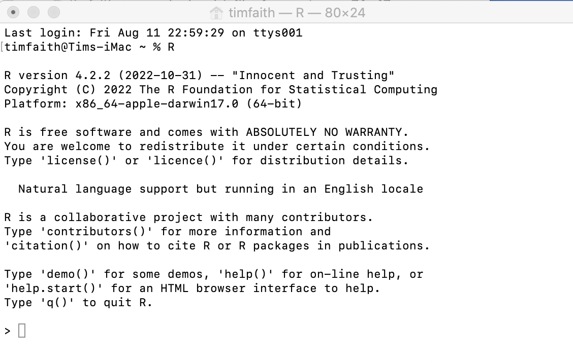
If all went well, R awaits your command (albeit, with ABSOLUTELY NO WARRANTY).
What happens next is entirely determined by your research questions. R is flexible. Numerous people far smarter than I have developed all sorts of statistical packages that you can import into R for analysis.
For some projects, a linear regression or a multi-variable linear regression model may be the tool that you need. R supports this through the lm and glm functions.
For other projects, your research may require a Preference Score Match approach. R supports this through the popular matchit library. Multi-level modeling is also supported through lme4. My guess is that if there is a statistical tool you need, someone has developed one for R that is available for import into your installation.
To get started with a particular package, be sure to install it in R as above in the Pre-requisites section. To use that package in a particular R session, use the library() command to load that package for your analysis:
library(RMySQL)
library(marginaleffects)
library(cobalt)
library(MatchIt)
library(lme4)
library(rbounds)
library(parallel)
library(ggplot2)
If you are missing a dependency, you can install that package if R doesn’t do it for you automatically with the install.packages command. Also, R is case sensitive, so RMySQL is not the same as rmysql.
From here, there are some steps you can take to analyze your data as follows:
- Connect to your MySQL database using the RMySQL library.
- Create a query object that R can use for analysis, passing a query for data to your database, and fetch the results into an object in R.
- Plot your data in various ways using ggplot to Quartz and export the charts you like into a .png file.
- Execute various analyses of your data using various statistical tools that meet your needs and report the results.
Here are some examples of commands you can execute in R for your analytical pleasure. Extensive documentation on options and switches are available from any web browser connected to the internet.
This first set of commands will connect you using the RMySQL package to your MySQL database. The data set that results from your query will reside in the mydata object:
conn=dbConnect(RMySQL::MySQL(),dbname=’MyData’,host=’localhost’,port=3306,user=’your_username_here’,password=’your_password’)
grades=dbSendQuery(conn, “select * from tbMyData”)
mydata=fetch(grades, n=-1)
You can create a scatterplot of your data if you want to compare two variables to look for relationships between them, such as student GPA and final course grade:
ggplot(d, aes(x=GPA, y=FinalGrade)) + geom_point() + geom_smooth(method = “lm”, se = FALSE) + labs(x=”GPA”, y=”Final Grade”, title=”Final Grades by GPA”)
You can export charts that you like from Quartz to an image file on your computer using the ggsave command:
ggsave(filename = “/path/to/save/your/image/figure1.png”, plot = figure1, width = 8, height = 11, dpi = 600)
You can create linear regressions of your data using lm. The basic syntax here is lm ( Dependent Variable ~ Independent Variables here separated by the plus (+) symbol, data=mydata)
m0=lm(FinalGrade~GPA+Inter+Race+Gender+Age, data=mydata)
summary(m0)
The summary command will then display a table of the results of your linear regression, giving you Residuals, Coefficients, Residual Error, Multiple and Adjusted R-squared, and F-statistic. Significant results are denoted with *** which suggests a very low probability of a chance relationship between the dependent and independent variable. Negative estimates suggest a lower FinalGrade for those variables, whereas positive estimates suggest a higher FinalGrade for those associated variables.

For the above analysis to work, some data manipulation is required to convert strings into numbers. For example, the Final Letter Grade could be converted into a number using a formula of A=4, B=3, C=2, D=1, FW=0, Male = 1 else 0, Race=’B’ then 1 else 0 in MySQL to build a view of your underlying data table.
create view vwMyData as select studentID, case when finalgrade=’A’ then 4 when finalgrade=’B’ then 3 when finalgrade=’C’ then 2 when finalgrade=’D’ then 1 Else 0 END as CodedGrade, Inter, GPA, case when Race=’B’ then 1 else 0 END as isAA, case when gender=’M’ then 1 else 0 END as isMale, Age from mngt140data;
Then, you can reload your data into R, using the view as your source rather than the underlying data table:
grades=dbSendQuery(conn, “select * from vwMyData”)
mydata=fetch(grades, n=-1)
Depending on the scope of your project, you may instead want to build a Preference Score Match-based (“PSM”) model for analysis of your data. For educational research, PSM may result in a more accurate analysis of instructional treatments because the matching methodology ensures that similar students are included in both your control and treatment groups, resulting in a more accurate Average Treatment Effect on the Treated (“ATE”) in the study.
Rosenbaum and Rubin (1983) originally developed the Propensity Score as expressed in the following formula: ei = P r (Zi = 1|Xi), where ei is the preference score of the individual, i, Xi is a vector of features or characteristics for individual i, and Zi is a binary variable indicating whether or not individual i is a match. The purpose of calculating a Propensity Score is to create a similar treatment and control group so that the distribution of known covariates is similar between the two groups (Austin, 2011). (“Thus, in a set of subjects all of whom have the same propensity score, the distribution of observed baseline covariates will be the same between the treated and untreated subjects.”) Several other researchers have discussed the use of PSM and MatchIt in R, including Griefer, 2022; Ho, et al., 2011; Zhao, et al., 2021; and Fischer, et al., 2015.
R supports a variety of PSM methodologies. This paper will focus on using MatchIt. One of the key issues for PSM is collecting relevant independent variables that may have a non-chance relationship to the dependent variable. Alyahyan & Dustegor’s research identified a substantial number of independent variables that may predict student performance based on the research of others (Alyahyan & Dustegor, 2020). As a practical matter, not all of these variables may be available to conduct matching, or the research sample may be too small to use all variables to match control and treatment units effectively. Some discretion must be exercised by the researcher to develop a meaningful and proper PSM model from the data available.
The syntax to build a PSM model is:
m0.out<-matchit(CodedGrade~Inter+GPA+isMale+isAA+Age, data=mydata, distance=’glm’, method=’exact’)
summary(m0.out)
plot(summary(m0.out))
MatchIt supports a variety of methods for matching control and treatment groups and which are discussed in more detail by Zhao, et al., 2021. In the example above, I have used the “exact” method, which requires that a control and treatment unit must essentially be identical to each other to be included in the match data. As a practical matter, this method may exclude too many treated units to result in a fair match, which is why the researcher should consider several possible matching methods for their analysis.
The plot of the summary of this model is a Love plot, which will help visually assess whether the model is appropriately balanced across all the independent variables used for matching. Generally, a balanced model would have an absolute standardized mean difference of less than 0.1 for all variables used to create the model.
If the model seems appropriately balanced, the next command creates a match object:
mdata0 <- match.data(m0.out)
From here, you can create a linear regression fit object, which can be fed into comparisons to calculate the ATT:
fit0 <- lm(CodedGrade ~ Inter+GPA+isMale+isAA+Age, data=mdata0, weights=weights)
comp0 <- comparisons(fit0, variables=”CodedGrade”, vcov=TRUE, newdata=subset(mdata0,CodedGrade==1), wts=”weights”)
summary(comp0)
The summary command of the comparisons object will give you a calculation of the ATT:

In this case, the ATT would be 0.0323 with a relatively low p value suggesting in our made up example that the treatment was highly correlated with an increase in student final grades when controlling for other variables included in the match object.
Parting Thoughts
The database administrator in me feels the need to recommend you backup your data stored in MySQL just in case you have a data disaster and need to recover from a checkpoint. A simple script you can run in Terminal will create a backup file of your MySQL database. You can also copy your python and R scripts to a cloud-based storage file just in case your computer fails you.

If you have created more than one database, you can add them in the DB_LIST variable separated by a comma, and the do loop will backup each one for you. Extra credit if you can find a way to schedule this script to run on a regular basis so you don’t have to think about backing up your data manually!
You can restore your databases from these backup files using the following MySQL command:
mysql -u username -p database_name < backup_file.sql
In sum, these open source tools can be employed to effectively analyze data for all sorts of interesting research questions. Happy querying!
FURTHER RESEARCH
Alyahyan, Eyman, Dustegor, Dilek (2020) Predicting academic success in higher education: literature review and best practices, 17 (3). https://doi.org/10.1186/s41239-020-0177-7
Austin, Peter C. (2011) An Introduction to Propensity Score Methods for Reducing the Effects of Confounding in Observational Studies. Multivariate Behavioral Research 46 (3): 399–424. https://doi.org/10.1080/00273171.2011.568786.
Fischer, L., Hilton, J., Robinson, T.J. (2015) A multi-institutional study of the impact of open textbook adoption on the learning outcomes of post-secondary students. Journal of Computing in Higher Education, 27, 159-172. https://doi.org/10.1007/s12528-015-9101-x
Griefer, Noah. (2022) MatchIt: Getting Started. https://cran.r-project.org/web/packages/MatchIt/vignettes/MatchIt.html#assessing-the-quality-of-matches
Ho, Daniel, Imai, Kosuke, King, Gary, Stuart, Elizabeth A. (2011) MatchIt: Nonparametric Preprocessing for Parametric Causal Inference. https://r.iq.harvard.edu/docs/matchit/2.4-20/matchit.pdf
Rosenbaum, P. R., and Rubin, D.B. (1983). The Central Role of the Propensity Score in Observational Studies for Causal Effects. Biometrika, 70(1), pp. 41-55. https://doi.org/10.1093/biomet/70.1.41
Zhao, Qin-Yu, Luo, Jing-Chao, Su, Ying, Zhang, Yi-Jie, Tu, Guo-Wei, and Luo, Zhe (2021) Propensity score matching with R: conventional methods and new features. Annals of Translational Medicine, 9(9), 812. https://atm.amegroups.com/article/view/61857
